Ring Attention Explained

By Kilian Haefeli, Simon Zirui Guo, Bonnie Li

Context length in Large Language Models has expanded rapidly over the last few years. From GPT 3.5’s 16k tokens, to Claude 2’s 200k tokens, and recently Gemini 1.5 Pro’s 1 million tokens. The longer the context window, the more information the model can incorporate and reason about, unlocking many exciting use cases!

However, increasing the context length has posed significant technical challenges, constrained by GPU memory capacity. What if we we could use multiple devices to scale to a near infinite context window? Ring Attention is a promising approach to do so, and we will dive into the tricks and details in this blog.

It took us a few tries to understand how Ring Attention works beneath its magic. Several tricks have to click in your head to really grasp it! In this blog, we will go through them step by step:

• We will build up why scaling long context across GPU is so challenging.
• Understand how we can divide up attention calculation across the sequence dimension into chunks.
• See how we can map the divided up attention calculation on multiple GPUs and orchestrate the computation in a way that adds minimal overhead, by cleverly overlapping communication and computation.

Notably the techniques we present here leading up to Ring Attention are general tricks to split computation of Attention into parallel parts. These techniques have been discovered by different amazing researchers and used in other transformer optimizations such as Self-attention does not need $𝑂(𝑛^2)$ memory. and Flash Attention. Note that these optimizations and ring attention are orthogonal concepts, in that they can be used independently from each other.

Attention and Memory

Why is long context so hard? Let’s look at computing attention in the transformer. We have query, key, value - each is a matrix of shape $s \times d$ - sequence length times model dimension. We need to compute $$O =\text{softmax}(QK^T)V$$, this looks like

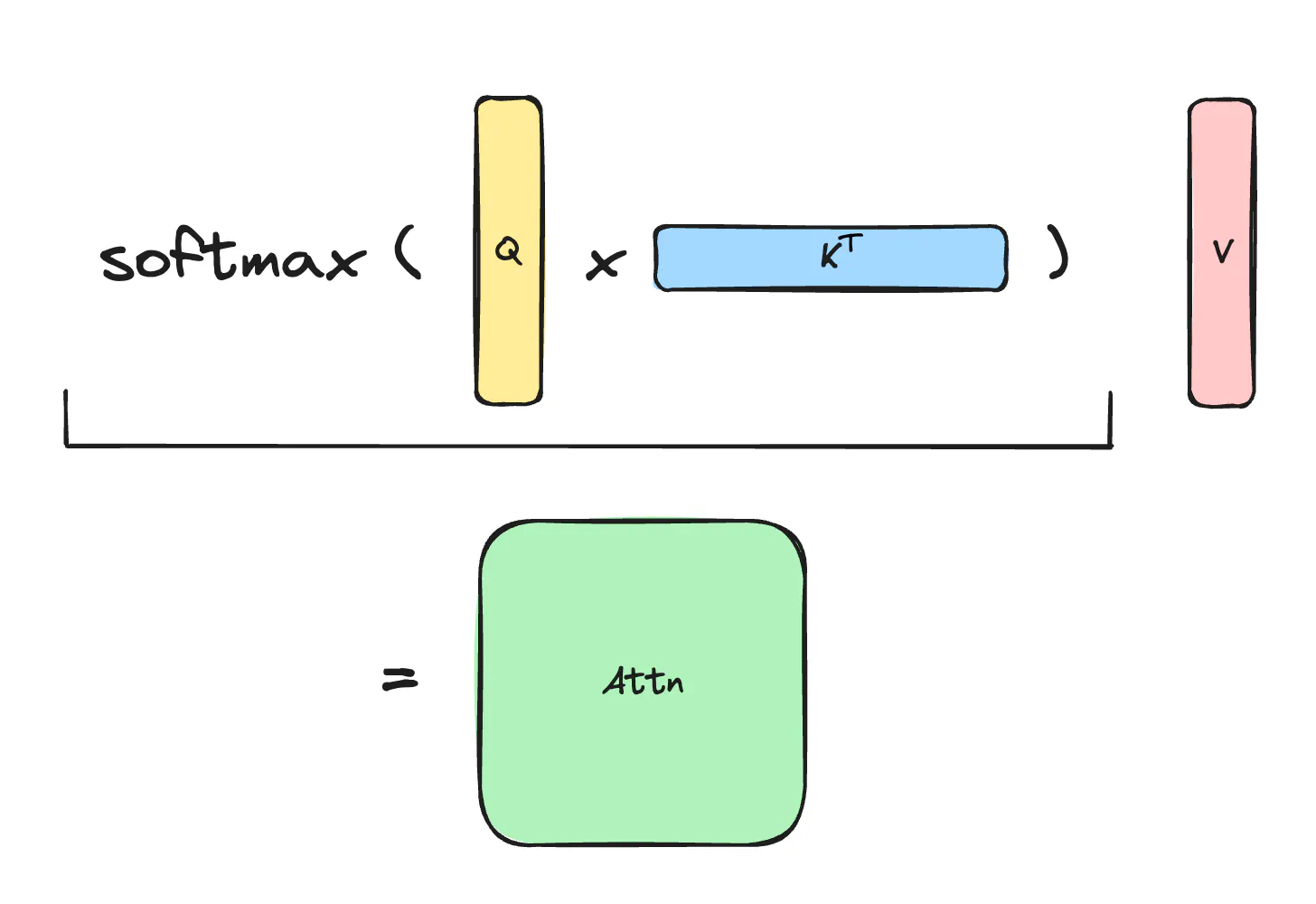
Notice that the Score Matrix $S=QK^T$ and the Attention Matrix $A=\text{softmax}(QK^T)$ are both of size $s \times s$, so the memory complexity of naive attention is quadratic with sequence length! Even using advanced optimizations like Flash Attention, the memory complexity is still linear in sequence length. Thus for long contexts, scaling the sequence length is limited by the memory capacity.

The goal of splitting the computation into parts is to split the memory cost, dominated by the sequence length, into parts which each require only a fraction of the total memory complexity. For N GPU’s, we want to split computation into parts each requiring 1/N’th of the whole memory cost. In order to achieve that, we need to split both Q and K, V along the sequence dimension.

However, to compute the final attention result, we still need to access all these matrices that are now split up across GPUs. Naively doing so could add a lot of communciation overhead especially as these matrices grow linearly with sequence length!

Ring Attention presents a way to cleverly to address this! A sneak peak of how this is going to play out: We will rotate between devices to parallelize all computation and hide the communication overhead completely. It looks something like:

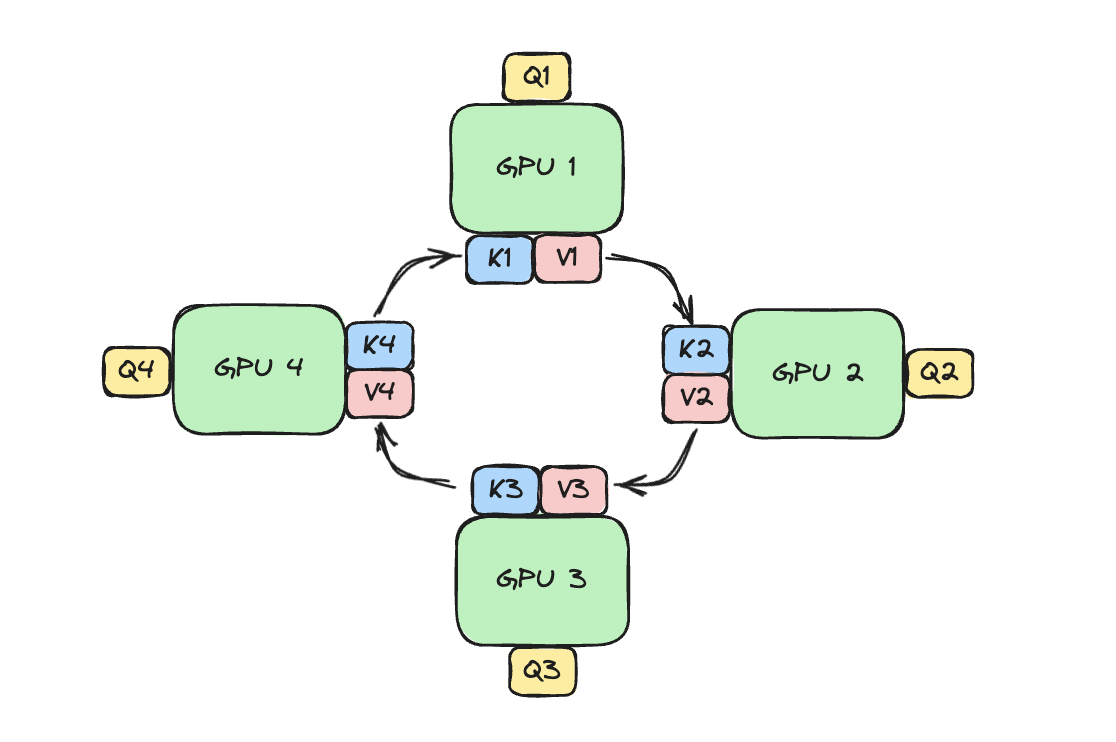GPUs are arranged in a ring, each holding a portion of the query. During the Ring Attention process, the GPUs will pass along blocks of K, V to each other; eventually each device will have seen all the blocks needed to compute attention output! We will show why and how this works in the rest of blog.

Splitting Q

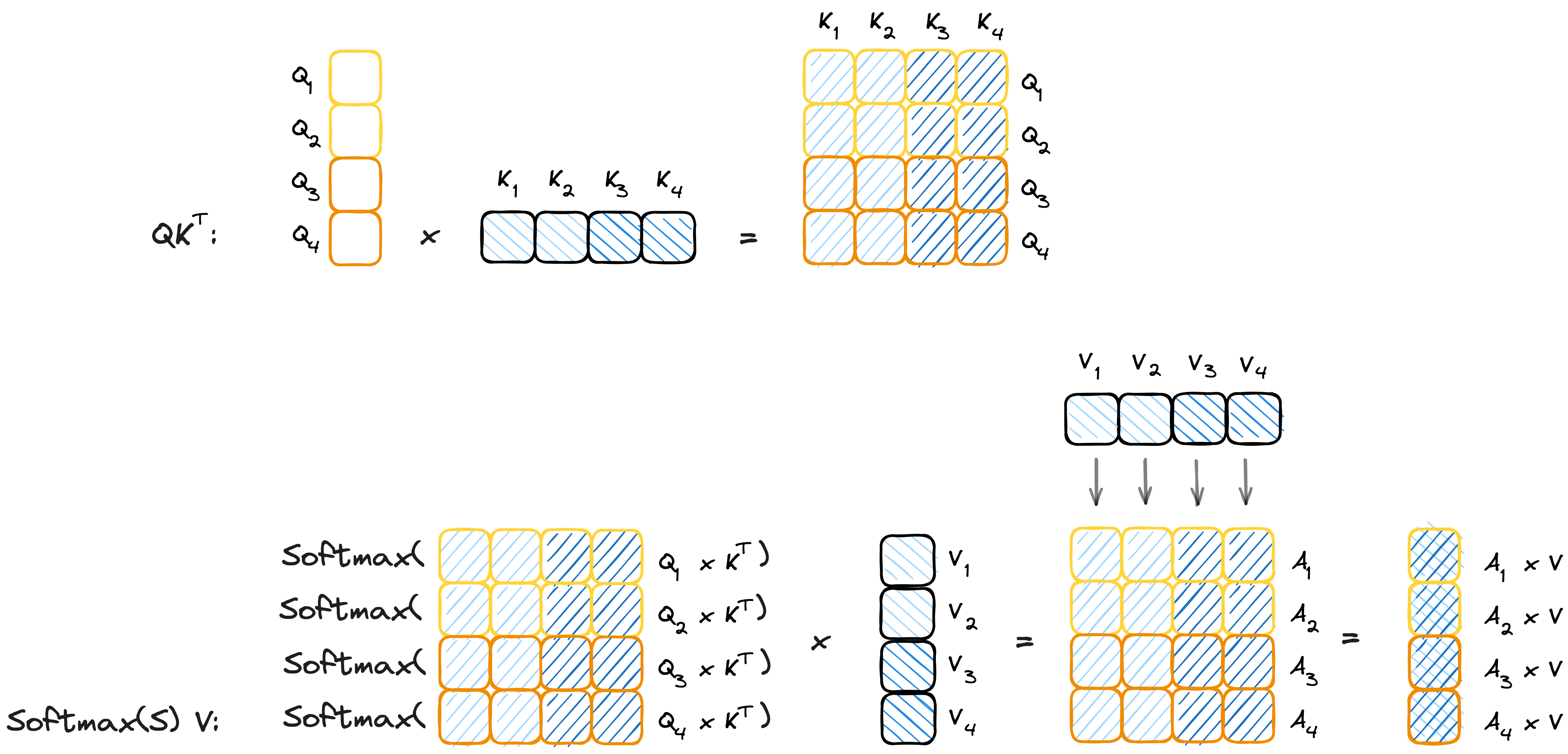
How can computation be split along the sequence length of $Q$? If you want to find out for yourself, follow the orange colours in the Attention visualization below. You will see that computation of each output row only depends on a single query row in $Q$. Assume we split $Q$ into $B_Q$ chunks of along its rows. Each $Q_i$ chunk is of the shape $C_Q \times d$, where $C_Q$ is the chunk size and $C_Q \times B_Q = s$. Let’s assign one such Query-chunk to each available GPU, what would each GPU need to compute attention? It still needs all of K and V! So far we did split the memory of $Q$ into $B_Q$ chunks, and the corresponding Score and Attention matrices are also split into $B_Q$ chunks. Now we need to split the keys and values.

Splitting K and V

How can we split up the sequence length for keys and values? Hint: It is not as trivial as splitting queries was!

Let’s look at the computation for a single Query chunk in the illustration above. What would happen if we additionally split the Keys along its rows (indicated by the blue colour)? Importantly note how the matrix multiplication $S=QK^T$ is now split along both rows and columns! The problem is that the Softmax operation needs to be computed over full rows of S at a time.

$$\text{softmax}(s_i) = \frac{\exp(s_i)}{\sum_{j=1}^{N}\exp(s_j)}$$

Don’t worry, we will see how we can work around this challenge. First we need to understand why the Softmax seems to require access to the whole row at once: Looking at the softmax equation, it is clear that the upper part of the fraction (numerator) does not need access to the whole row at once as it simply takes the exponent of each individual entry. The lower part of the fraction however requires you to compute the sum of ALL elements in the row - at least that is how it seems upon first inspection ;)

We will later see how we can handle the lower part (denominator) of softmax in a parallel fashion, but for now imagine that the lower part simply does not exist.

We already know that we can easily partition computation along the rows (sequence dimension) of $Q$. Hence, here we partition the computation of a single $Q_i,A_i$ chunk into $B_{KV}$ independent sub-parts involving only a single $K_j, V_j$, $j\in{1,…,B_{KV}}$ chunk at each step. The computation of a single Query, Output chunk $Q_i,A_i$ is:

This directly leads to our desired result! Computation is now split into an outer loop over $B_Q$ chunks of $Q$ and over an inner loop over $B_{KV}$ chunks of $K$ and $V$. At each step we compute only $\exp(Q_iK_j^T)\cdot V_j \in R^{h\times c_Q}$ which requires only single chunks of $K_j$, $V_j$ and $Q_i$ at a time, successfully dividing memory cost over the sequence length (Setting the number of chunks to $N$ ($B_{KV}=B_Q=N$) would result in $1/N$th of the memory complexity of stoing the full $K,V,Q$).

Put it in a Ring: We have the outer loop (parallel over Query chunks) and inner loop (parallel over Key and Value chunks). But how are the computation steps of this loop allocated to the devices?

Note how the outer loop can be computed completely independently, whereas the inner loop calculates a sum of its results. We partition computation to devices in the following way: Each device gets one $Q_i$ chunk (one outer loop index) and calculates the inner loop iteratively for each $K_j,V_j$. Each device at a given step $j$ only needs to keep track of the cumulative sum $A_i$ of shape $h\times c_Q$ and only needs a single $V_j, K_j$ block at a time, along with its $Q_i$. Therefore the memory requirement for each device is successfully split, even for $K$ and $V$.

Online softmax

Now let’s look at the normalization constant, how can we compute normalization constant on each device with just local results?

There is a simple solution! We accumulate the partial sum $l^{j}=l^{j-1}+\sum_{k_t\in K_j}\exp(Q_i k_t^T)$, every time we receive a key and value chunk. By the end of the inner loop, the device would have accumulated $l=l^{B_{KV}}=\sum_{j=1}^{s} \exp(Q_i k^T_j)$, which is the normalization constant we need. Note that the order of normalizing and multiplying with the value matrix V does not make a difference, which is why we can accumulate the sum and execute the actual normalization after everything else.

Therefore each device $i$ (holding $Q_i$), additionally to its cumulative sum $A^{j}=A^{j-1}+\exp(Q_iK_j^T)V_j$, also keeps track of its current $l^{j} \in \mathbb R^{B_Q}$, while executing the inner loop. At the end of the inner loop, each device finishes by dividing its computed unnormalized Attention by the normalization constant $A^{B_{KV}}/l^{B_{KV}}$.

Safe softmax

The exponential operation can easily grow out of bounds, leading to numerical issues and overflow. Typically to compute softmax, we subtract the maximum from every element. That is

$$\text{softmax}(s_{1:N}) = \frac{\exp(s_{1:N})}{\sum_i{\exp(s_i)}} \cdot \frac{\exp(- s_{max})}{\exp(- s_{max})} = \frac{\exp(s_{1:N} - s_{max})}{\sum_i{\exp(s_i - s_{max})}}$$

This is called the safe softmax. How can we subtract the maximum when we are computing the softmax in blocks? We can keep track of the maximum so far. Let’s say our current sum is $A^{j}$ and current maximum is $m^{j}$, we receive a new key $K_{j+1}$ and value $V_{j+1}$, we compute $Q_iK^T_{j+1}$ and get a new maximum $m^{j+1}=\max(m^{j},\max(Q_iK^T_{j+1}))$, we can update our result as:

$$A^{j+1} = A^{j} \cdot \exp(m^{j} - m^{j+1}) + \exp(Q_iK^T_{j+1} - m^{j+1}) \cdot V_j$$

$$l^{j+1} = l^{j} \cdot \exp(m^{j} - m^{j+1}) + \exp(Q_iK^T_{j+1} - m^{j+1})$$

To conclude: For an inner step $j+1$, before computing the cumulative sum $A^{j+1}$ and the normalization constant $l^{j+1}$ we first compute the current maximum $m^{j+1}$, then renormalize the previous $A^{j},l^{j}$ using our newfound maximum and finally compute the updated $A^{j+1},l^{j+1}$.

Putting it together

Finally, we have assembled all the tools we need to construct ring attention:

1. Splitting along the sequence length of $Q$ into an independent outer loop.
2. Applying online safe softmax in order to split along the sequence length of $K$ and $V$ resulting in an inner loop computing the attention cumulatively.

As hinted on before the way this is parallelized is by assigning each of the N devices available one chunk $Q_i$ of $Q$. Therefore we need to split $Q$ into N equal parts ($B_Q = N$). Each device will individually compute its output block $Output(Q_i, K, V)=\text{softmax}(Q_iK^T)V$ iteratively by performing the inner loop over the blocks of Keys and Values. The challenge is that the devices are not able to store the full K and V matrices at a time.

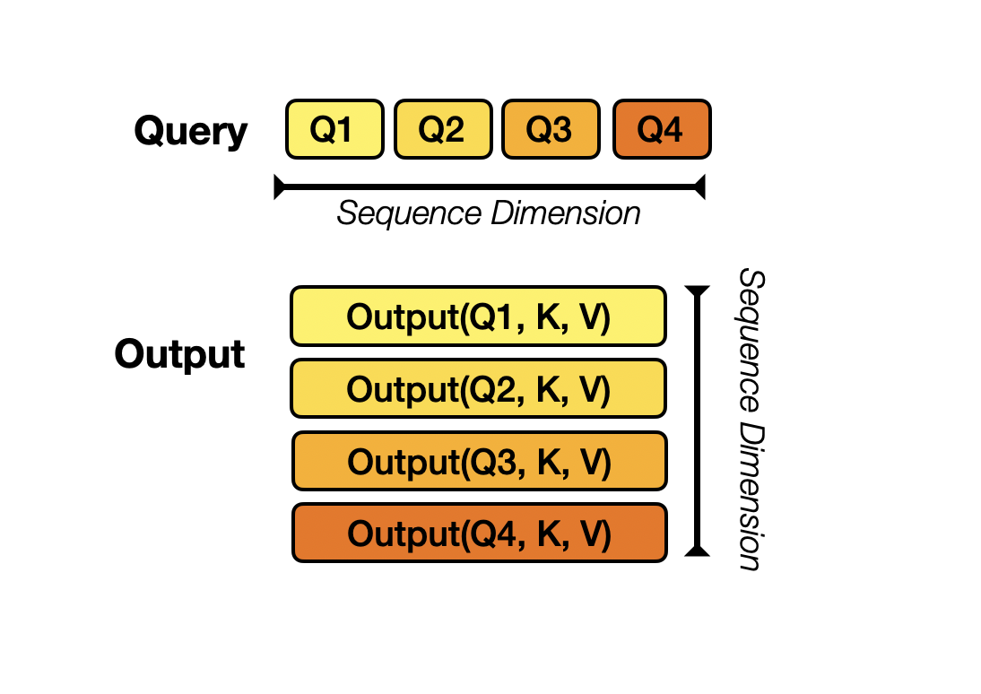For example if we have 4 GPUs, we will split Query into 4 blocks along sequence dimension for each device. Each device would then compute output using local Q and the whole K, V. The final output would be concatenation of these local outputs along row-dimension

Remember how we showed that we can further split K, V as the inner loop? K and V are now split into $B_{KV}=B_Q=N$ blocks and initialize the devices so that each device holds a single $Q_i$ block and a single Key $K_j$ block and Value $V_j$ block. For simplicity we can assume that device $i$ holds $Q_i,K_{j=i},V_{j=i}$ in the beginning.

After the devices have computed one inner loop step corresponding to their current $V_j, K_j$, each device needs to receive a next Key and Value block to continue the inner loop. Sending and waiting for these matrices is a big overhead that we do not want to wait for! This is where the ring in Ring Attention comes into play: We lay out the N devices in a ring, where device $i$ can send data to device $i+1$ and so on as illustrated:

Observe that for GPU1, while it is computing output using $Q_1$ (its local query) and $K_1$, $V_1$ (the local K,V blocks that it currently has), it is also receiving $K_4$, $V_4$ from GPU4 (previous host int the ring) and sending $Q_1$, $V_1$ to GPU2 (next host in the ring). The network communication are illustrated by the blinking arrows. If we select the block size correctly, by the time GPU1 has computed output using $Q_1$, $K_1$, $V_1$, it has received the block $K_4$, $V_4$ to compute the output in the next iteration!

Computing a step of the inner loop on device $i$: $Q_i, V_j, K_j$ takes a certain amount of time. If during that time the device $i$ can also send its current $V_j, K_j$ to device $i+1$ and simultaneously receive $V_{j-1}, K_{j-1}$ from device $i-1$, then the latency from sending and receiving the Key and Value chunks is hidden behind executing the actual computation, as long as the time to transmit is lower than the time it takes to compute. We now can completely hide the communication overhead!

Here we illustrate for $N$ devices, it will take $N$ iterations to finish the whole output comptutation. Watch for each iteration on each device, different partial sum of the output is computed with the K,V block it currently has, and it eventually sees all the K,V blocks and has all the partial sum for the output!

Memory and Arithmetic Complexity

For this analysis we will use the bfloat16 format that is commonly used in deep learning applications. Parallel processing accelerators such as GPU’s or TPU’s are usually measured by their FLOPs$:=F$, which is the number of floating point operations the device can theoretically execute per second. In practice, we never really see full utilization but for the sake of this analysis we will assume that. Furthermore, the connections between the different devices we assume to have bandwidth $:=B \frac{\text{Bytes}}{\sec}$.

Memory Complexity: In order to receive send and compute at the same time we need to have memor for receiving the new Key Value blocks. Storing the current Key Value blocks requires $2 \cdot d \cdot c$ floats or $4 \cdot d \cdot c$ Bytes. The memory for receiving the new Key Value blocks is also of size $2\cdot d\cdot c$ floats or $4 \cdot d \cdot c$ Bytes. Now assuming that the computation itself does not require more memory (this would require a more in depth discussion, but there are ways to do this like flash attention or blockwise attention) computing the output of the current step requires $d \cdot c$ floats or $2 \cdot d \cdot c$ Bytes. Furthermore each device needs to store its $Q_i$ block which also takes $d*c$ floats or $2 \cdot d \cdot c$ Bytes. In total we require $6\cdot d\cdot c$ floating points or $12 \cdot d \cdot c$ Bytes of memory.

• A note for people familiar with Flash Attention: Ring Attention is an orthogonal concept to things like flash attention and could be used together (Flash attention is actually used in the inner loop of Ring Attention). These latter methods have the goal of not materializing the full Attention matrix and thus getting linear memory complexity in sequence length vs quadratical like the naive implementation would. Ring Attention manages to split memory complexity for both the naive and the flash attention method by at least $N$ times using $N$ devices, because it splits everything into at least $N$ or more parts (Splits Keys, Queries and Values into $N$ parts, and splits the Attention Matrix into $N^2$ parts)! No matter whether the memory complexity is dominated by the Keys, Queries and Values or by Attention Matrix, Ring Attention manages to split memory cost by at least $N$ times.

Communication Complexity: During a single step, each device needs to send $2 \cdot c_Q \cdot d$ floating point values, from $K_j, V_j \in \mathbb{R}^{c_Q \cdot d}$, to the next device over a channel with bandwidth B. Each floating point value consists of two Bytes. Thus the time it takes to transmit both is approximately $4 \cdot c \cdot d/B$

Arithmetic Complexity: Computing an inner loop step requires $2\cdot d\cdot c^2$ for computing $Q_iK_j^T$, $2 \cdot c \cdot d$ for computing the softmax along with the $l^{j}_i,m^{(j)}_i$ normalization and safety parameters, and $2\cdot d\cdot c^2$ for computing $A_i^j \cdot V_j$. Assuming that the device operates at the maximum possible FLOPs (in reality we would use the achieved average FLOPs) the time it takes to compute is roughly $\approx 4 \cdot d \cdot c^2/F$

In order to effectively overlap the communication and computation (aka hiding the commmunication overhead), we need the time of transmission of K, V blocks equal to the time it takes to compute the local Q, K, V : $$4 \cdot c \cdot d/B \leq 4\cdot d\cdot c^2/F \iff B\geq F / c \iff s/N\geq F/B$$

Further optimizations

One interesting case of Ring Attention is when used for causal transformer models, recall the triangular mask is used for attention calculation. This implies that some GPUs won’t need to compute over the whole sequence, which results in them being idle for the most part. An extension of Ring Attention, Striped Attention addresses this constraint and provides a scheme to distribute computation more even and hence making Ring Attention even faster!

Besides technniques like Ring Attention and Flash Attention to enable the standard Transformer architecture to have longer context length, there are also attempts to experiment with model architecture such as state space models (SSMs) with linear attention such as Mamba, but that is a deepdive for another day.

Summary

So let’s review how we arrived at this magical zero-overhead solution:

1. Attention requires quadratic memory (or linear if optimized) in the sequence length. Scaling transformers to any desired sequence length therefore requires splitting memory cost over several devices, and we want do that in a low-overhead manner.
2. We want to parallelize the attention calculation, as well as the shard the $Q, K, V$ matrices across devices because they grow linearly with the sequence length.
3. One particular way is to shard on the sequence dimension for Query as blocks, but each sharded query each still needs to compute with all the $K,V$’s (which can be huge)!
4. We show that it is possible to further parallelize softmax calculation by creating an inner loop over $K,V$, with the correct normalization to recover the final softmax! This leverages the fact that the operations are commutative and all we need to do is cumulatively sum up the normalization, whilst also keeping track and renormalizing with the current maximum.
5. Ring Attention builds on this technique of parallelizing Attention calculation by distributing the outer loop over $Q$ blocks to the individual GPU’s, while letting the inner loop be computed in a ring-reduce fashion. Instead of waiting for new Key, Value blocks we effectively hide transmition overhead by “rotating” the Key, Value blocks in a ring around the devices to compute the partial sums. With the correct block size, we can overlap communication with computation and fully hide overhead induced by communication.

Acknowledgement

We like to thank Jay Alammar and Bowen Yang for their insights! We also like to thank Daanish Shabbir, Yuka Ikarashi, Ani Nrusimha, Anne Ouyang, for their helpful feedback!

---